Virginia’s Eastern Shore Hedging Simulation

The farmer in this simulation works 1,000 acres and utilizes a typical Virginia crop rotation of corn-wheat-soybeans. We assume that the farmer splits his/her production each growing season into equal halves by simultaneously growing 500 acres of corn and 500 acres of soybeans. Once the corn is harvested in the fall, the farmer will then sow 500 acres of winter wheat. The Eastern Shore of Virginia was chosen for this simulation due to the abundance of price and basis data, the same simulation could be conducted with other locations in Virginia, however they may have missing data. The hedging simulation compares two common marketing strategies used by Virginia producers, selling at harvest in the cash market and hedging with futures during the growing season followed by selling grain in the cash market during harvest. In order to calculate the expected production for the simulation, the most recent five-year average yield for each crop in Virginia was calculated using yield data obtained from NASS. Once the expected yield was calculated, it was multiplied by the acres grown to give an expected production. This simulation was conducted using data from 2000-2021.

The first strategy simulated is selling strictly in the cash market at harvest. It assumes that the farmer sells 25% of their production of each crop each week throughout the harvest month (October for corn and soybeans and June for wheat). Cash prices were collected directly from the VDACS Market News Service. The cash prices were then multiplied by the bushels sold for the week to give a gross income for the week. The four weeks in each harvest month were then added together to form a gross income for each year, since it is assumed that the entire crop is sold during the harvest month.

The second strategy simulated is hedging 75% of the farm’s production with the futures market during the growing season. For corn, a December corn futures contract was sold each week in April, May and June until 12 contracts were sold. For soybeans, one November soybean futures contract was sold in the first week of April, May, and June, for a total of three contracts. Finally, for wheat, one July Chicago wheat futures contract was sold in the first week of October, then one contract was sold in the first two weeks of November and December for a total of five contracts. The farmer holds the short futures positions until harvest and then the farmer gradually buys back the contracts as they sell their grain in the cash market. The farmer buys back three corn contracts each week in October for a total of 12 contracts, one soybean contract for the first three weeks in October for a total of three contracts, and one wheat contract each week in June and the first week in July for a total of five contracts. The difference between the buy and sell prices of each contract are calculated and summed up for each commodity for each year. This value shows the gain or loss in the futures market for each year. Then, those gains or losses are added to the income from the cash sale shown in the first simulation to give the total gross income for the simulation using the futures market.

Figure 1 shows the Eastern Shore corn hedged vs. unhedged simulation results from 2000 to 2021. The maroon line indicates the unhedged scenario while the orange line indicates the hedged scenario. There are two main takeaways from this figure. The first is that the hedged scenario produced a higher return or gross income in 17 of the 22 years that were calculated. The second takeaway is that the hedged values were much less volatile and show less volatile swings than the unhedged values.

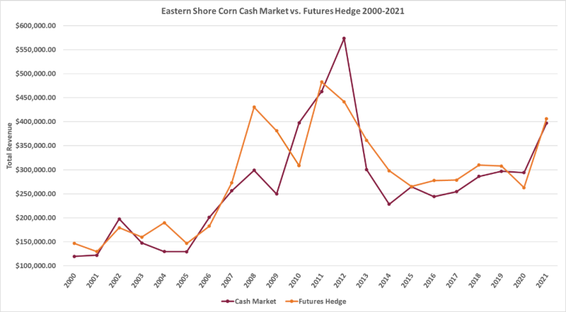
Figure 2 shows the Eastern Shore soybean hedge vs. unhedged simulation results from 2000 to 2021. In the soybean simulation, the hedged scenario produces higher returns or higher gross income in 12 of the 22 years. The hedged scenario also seems to exhibit less volatility than the unhedged scenario, just as we saw in the corn simulation. While this soybean simulation suggests similar results as the corn simulation, the two scenarios are much closer and don’t exhibit some of the wider differences that were observed for corn.

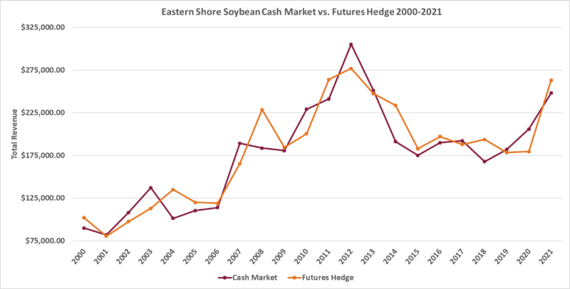
Figure 3 shows the Eastern Shore wheat hedge vs. unhedged simulation results from 2000 to 2021. In the wheat simulation, the hedged scenario produces higher revenues in 14 of the 22 years. When looking at the revenue volatility of these two scenarios, the results seem to differ from those observed in the corn and soybean simulations. It looks as if for wheat, there is volatility present in both scenarios. Another interesting trend to point out is that the wheat hedger outperformed the unhedged scenario every year from 2009 to 2016. 

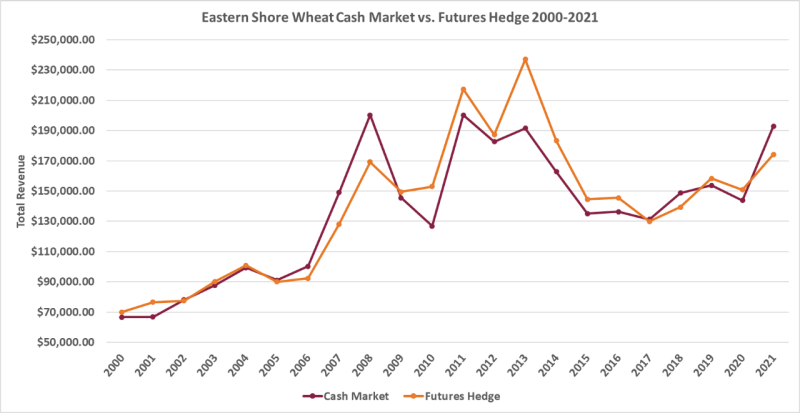
Table 1 shows the cumulative revenue calculations from the simulated scenarios. In each simulation, the hedged scenario produces more gross income than the unhedged. The corn hedge produced much higher returns over the 20-year period when compared to wheat and soybeans. However, soybeans and wheat still saw positive returns which shows potential for growers of those crops as well. Also, when the results for all three crops are added together, the hedged producer had just over a half million dollars of additional revenues over the past 20 years, a number that could have a large impact on a farming operation. A key question a producer should think of asking is: How much different would my operation look if it made just over a half million more dollars in the past 20 years?  However, it is important to keep in mind that these results do not include transaction and margin account fees described in the Margin Account Section.

Table 1: Cumulative Revenues from the Eastern Shore Hedging Simulation over 2000-2021

Table 2 shows average annual returns for the three commodities included in the Eastern Shore Hedging simulation. These calculations offer a different look at the profitability of the hedges as they show what a producer could expect on a yearly basis on average. The corn hedge shows an average yearly return of $16,668 while soybeans and wheat offer just under $3,500 in average yearly returns. These add up to almost $23,500/year. This extra income can pay huge dividends to any operation, but especially smaller or struggling outfits with profit margins narrowing.

Table 2: Average Annual Revenues from the Eastern Shore Hedging Simulation over 2000-2021

While the additional revenues demonstrated above are always nice, the main goal of hedging is to reduce variability of returns, or price risk. Agricultural producers are subject to a considerable amount of price risk due to the volatility of grain prices. In order to test the volatility of the cash market revenues versus the futures hedging scenario, a simple standard deviation was calculated for each commodity and scenario. The standard deviation measures the extent of scattering in annual revenues, compared to the mean values shown in Table 3 (Amda and Sergent 2022). Table 3 shows that for corn and soybeans, the standard deviations for the futures hedge were lower than the cash market standard deviation and therefore have a negative difference. This suggests that the futures hedge mitigated price risk for the market participants. When looking at the wheat simulation, we see the exact opposite. The standard deviation for the cash market was lower than the one for the futures hedge. This is an interesting result and would suggest that the futures hedge is more volatile for wheat and adds more price risk to the producer. 

Table 3: Standard Deviation Results for the Eastern Shore Hedging Simulation from 2000-2021

While the results presented so far suggest that hedging results in slightly higher average annual revenues, it is important to recognize variability in revenues around these averages.  This means some years will have revenues that are slightly higher and other years will have revenues that are slightly lower than average. A two-tailed t-test allows comparing average annual revenues from two simulation scenarios while taking this variation into account (Wadhwa and Marappa-Ganeshan 2022). Table 4 shows the test statistics and p-values for each commodity being much higher than the 0.05 value that would indicate statistical significance at the 95% level. Thus, these results suggest that the annual average returns from two scenarios are not significantly different from each other. However, the economic significance is still present. Looking back to Table 2, the hedging strategy provides a half million dollars more of cumulative revenues to the farm over a 20-year period, a statistic that any farmer or producer would welcome to their operation. 

Table 4: Statistical Comparison of Average Annual Revenues from the Eastern Shore Hedging Simulation over 2000-2021

Variability in annual revenues across hedged and unhedged scenarios was compared using, a one-tailed f-test was used. An f-test is used to test if two population variances are equal or not (Shafer and Zhang 2022). Table 5 shows the test statistics and p-values for each commodity with all p-values exceeding 0.05, which would indicate significance at the 95% level. Thus, our findings suggest that annual revenues from the hedged and unhedged scenarios have similar variability. Even though the results of the standard deviation calculations are not statistically different, the standard deviations do show that while the difference is small, futures hedging for corn and soybeans reduces the price risk seen by the producer. 

Table 5: Statistical Comparison of Variation in Annual Revenues from the Eastern Shore Hedging Simulation over 2000-2021

It is important to note that transaction costs, commission, interest, and margin account fees are not included in these numbers and will need to be considered if a farm adopts a futures hedging strategy. In general, for each commodity, the hedged scenario showed higher gross profits more than 50% of the time. Also, there was a trend observed, more noticeable in the corn and soybean simulation than the wheat, but the hedged scenario tends to experience less volatile movements and swings from year to year. These observations are important because they can help us see the benefits of hedging.

If we think back to the definition of hedging, we find that hedging is the process of protecting against loss by making an equal and opposite transaction. This is important because the object of hedging isn’t to have the highest gross income, but to reduce price risk. In this example, we see that hedging in most cases reduced some of the price risk that producers are challenged with constantly. It also helps that this example shows more returns from the hedging scenario. This will differ between different strategies and locations and may not always show positive returns across each of the three commodities. However, the risk reduction that hedging offers may outweigh the losses that occur with the hedging strategy. The important thing to remember is that risk reduction is an essential part of a marketing plan. If a farm can reduce the price risk while making more gross income, then it is a win-win situation for the farm. Even if the gross income suffers from hedging, the farm manager has to calculate and know what the risk reduction is worth to their operation.

El Omda S, Sergent SR. Standard Deviation. [Updated 2022 Aug 22]. In: StatPearls [Internet]. Treasure Island (FL): StatPearls Publishing; 2022 Jan-. Available: https://www.ncbi.nlm.nih.gov/books/NBK574574

Shafer, D., & Zhang, Z. (2022). Introductory statistics. 

Wadhwa RR, Marappa-Ganeshan R. T Test. [Updated 2022 Jan 19]. In: StatPearls [Internet]. Treasure Island (FL): StatPearls Publishing; 2022 Jan-. Available: https://www.ncbi.nlm.nih.gov/books/NBK553048

Comparing Corn Marketing Strategies
Gloria Lenfestey and Michael Langemeier
Center for Commercial Agriculture
Purdue University, July 19, 2023